Decision Tree

So far we have covered linear regression and logistic regression which are limited to linear relationships. In contrast, decision trees are non-linear models able to capture complex relationships in the data. They are easy to interpret and visualize, making them a popular choice for many applications.

Moreover, decision trees can be used for both regression and classification!

In this chapter, we will explore the theory behind decision trees followed by practical examples. As always we will use scikit-learn for hands-on experience.

Basic intuition

Although you might not know it, you're already familiar with decision trees. Imagine, you're planning a skiing trip and need to decide whether to go skiing or not. You might ask yourself:

graph TD
    A[Can I get to a skiing resort?] -->|Yes| B[Is there any snow?]
    A -->|No| C[No skiing 😥]
    B -->|Yes| D[Go skiing ⛷]
    B -->|No| E[No skiing 😥]

    style A fill:#1e2129,stroke:#ffffff
    style B fill:#1e2129,stroke:#ffffff
    style D fill:#009485,stroke:#ffffff
    style C fill:#e92063,stroke:#ffffff
    style E fill:#e92063,stroke:#ffffff

Depending on the answers, you can decide whether to go skiing or not.

A decision tree resembles a flowchart where each internal node represents a decision based on a feature (e.g., Is there any snow?), each branch represents the outcome of that decision, and each leaf node represents a final prediction (either a class label for classification or a continuous value for regression).

To get a better understanding of the terms node, branch and leaf, consider the illustration of a (rotated) tree.

The same decision tree with literal illustrations of node, branch and leaf.

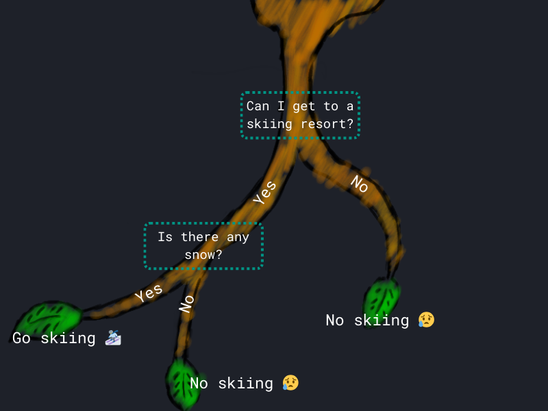
In the skiing example, the nodes are the questions you ask yourself. With branches being a simple binary split (the answers to the question). The leaf nodes are the final predictions, in our case whether to go skiing.

Given the skiing decision tree, what kind of supervised learning task is this?

Multi-class classification (not previously covered)

Regression

Binary classification

It's not a supervised learning task, since we are missing our target.

Submit

Correct, the leaves predict two different labels, namely "Go skiing" and "No skiing" which is a classic binary classification task.

Excited for some theory?

Theory

Info

This theoretical section on decision trees follows: Christopher M. Bishop. 2006. Pattern Recognition and Machine Learning¹

We focus on a particular algorithm called CART (=Classification And Regression Trees). The theoretical foundations of CART were developed by: Leo Breiman, Jerome Friedman, Richard Olshen, and Charles Stone. 1984. Classification and Regression Trees²

---

When building a decision tree a couple of questions arise:

• Question

  ---

  1. How do we pick the right feature for a split?
  2. What's the decision criteria at each node?
  3. How large do we grow the tree?

• Intuition

  ---

  1. Which questions do we ask? Why did we ask "Can I get to a skiing resort?" and "Is there any snow?"?
  2. It does not have to be a simple yes/no question. It can be a threshold for continuous values as well. E.g., "Is there more than 10cm of fresh snow?" But how do we choose the threshold?
  3. How many questions do we ask? Why only 2 and not more?

With these questions in mind, let's dive into the theory of decision trees in order to tackle them.

---

Greedy optimization

As a decision tree is a supervised learning algorithm, the goal is to predict the target variable \(y\) with a set of features \(x_1, x_2, ..., x_n\).

With the data at hand, the CART algorithm finds the optimal tree structure that minimizes the prediction error. In turn, the optimal tree structure depends on the chosen splits.

Info

A split in CART is a binary decision rule that divides the dataset into two subsets based on a specific feature and threshold.

Imagine if we extend our skiing example with the split "Is there more than 10cm of fresh snow?". The split divides the data into two subsets: one where observations have more than 10cm of fresh snow and another where observations don't. With amount of fresh snow being the feature and 10cm the threshold.

However, given large data sets, there are simply too many splitting possibilities to consider at once. Hence, the tree is grown in a greedy fashion.

The greedy optimization starts with a single root node splitting the data into two partitions and adds additional nodes one at a time. At each step, the algorithm chooses a split using exhaustive search. The best split is determined by a criterion. Remember, that decision trees can deal with regression and classification problems. Hence, the criterion differs for the two tasks.

---

Regression

For regression trees, the best split (feature threshold combination) at each node is determined by minimizing the residual sum-of-squares error (RSS), defined as:

Residual sum-of-squares (RSS)

\[ RSS = \sum_{i \in t_L} (y_i - \bar{y}_L)^2 + \sum_{i \in t_R} (y_i - \bar{y}_R)^2 \]

where \(t_L\) and \(t_R\) are the left and right child nodes after the split, and \(\bar{y}_L\) and \(\bar{y}_R\) are the mean target values in the respective nodes.

The algorithm searches through all possible splits to find the one that minimizes this RSS criterion.

Info

Since each split separates the input data into two partitions, the prediction is the mean of the target variable \(y\) in the respective partition.

Hence, intuitively speaking, we do not optimize the entire tree at once but rather optimize each split locally.

Classification

For classification tasks, the best split at each node is determined by minimizing the Gini impurity.

Gini impurity

For a node \(t\) with \(K\) classes, the Gini impurity is defined as:

\[ Gini(t) = \sum_{k=1}^K p_{k}(1-p_{k}) = 1 - \sum_{k=1}^K p_{k}^2 \]

where \(p_k\) is the proportion of class \(k\) observations.

The Gini impurity (sometimes referred to as Gini index) encourages leaf nodes where the majority of observations belong to a single class.

Info

The prediction at each leaf node is the majority class among the training observations in that node.

---

TLDR

No matter the task (regression or classification), with a greedy optimization strategy, the CART algorithm searches for the best split using an exhaustive search at each node to ultimately minimize the prediction error. Thus answering the first two questions, a (How do we pick the right feature for a split?) and b (What's the decision criteria at each node?).

A CART can be seen as a piecewise-constant model, as it partitions the feature space into regions and assigns a constant prediction (either the mean of a continuous value or a label) to each region.

Tree size

Lastly, we answer question, c (How large do we grow the tree?). Put differently, when should we stop adding nodes?

First, the tree is grown as large as possible until a stopping criterion is met. This criterion can be the maximum tree depth or a minimum number of observations per leaf. Second, the tree is pruned back. Pruning is the process of removing nodes that do not improve the model's performance. It balances the RSS error or Gini impurity against model complexity.

Info

If you want to dive deeper into tree pruning, we recommend reading page 665 of Bishop's book Pattern Recognition and Machine Learning¹

---

Advantages and Limitations

Decision trees offer several significant advantages, but they also have their limitations:

• Advantages

  ---

  • Easy to interpret and visualize
  • Can capture non-linear relationships

• Limitations

  ---

  • Prone to overfitting, i.e., building a model that perfectly fits the training data but fails to generalize on new (unseen) data.
  • Sensitive to data, i.e., small changes in the data can lead to significantly different trees.

Examples

As mentioned earlier, we will use scikit-learn for hands-on experience. scikit-learn contains an implementation of the CART algorithm discussed.³

Functionalities around decision trees are all part of the tree module in scikit-learn.

Regression

First, we start with a regression task. We will use the California housing data to predict house prices using a decision tree regressor.

Load data

Load the data and split it into training and test sets. If you need a refresh on training and test splits, visit the Split the data section of the previous chapter.

from sklearn.datasets import fetch_california_housing
from sklearn.model_selection import train_test_split

X, y = fetch_california_housing(return_X_y=True, as_frame=True)

X_train, X_test, y_train, y_test = train_test_split(
    X, y, test_size=0.2, random_state=42, shuffle=True
)

As always, a seed is set for reproducibility (random_state=42). It can be any integer, you can simply pick any number.

Fit and evaluate the model

Next, we load the class DecisionTreeRegressor from the tree module.

from sklearn.tree import DecisionTreeRegressor

model = DecisionTreeRegressor(random_state=784)

Again, we set a seed, as the tree's construction involves randomness.

To fit and evaluate the model:

model.fit(X_train, y_train)
score = model.score(X_test, y_test)
print(f"Model performance (R²): {round(score, 2)}")

>>> Output

Model performance (R²): 0.61

The score() method returns the coefficient of determination \(R^2\). You should be already familiar with \(R^2\), as it was first introduced in the Regression chapter to evaluate the fit of a linear regression.

The decision tree model achieved an \(R^2\) of 0.61 on the test set, which leaves room for improvement.

Info

On a side note: Although we fitted a decision tree on 16512 observations, the process of actually training the model is quite fast!

Plot the tree

It's a mess...

As discussed, one main advantage of decision trees is their interpretability. We can easily visualize the tree using the plot_tree function.

Tip

This is the first time that we discourage you from running the code snippet below. Soon you will know why.

import matplotlib.pyplot as plt
from sklearn.tree import plot_tree

plot_tree(model)
plt.show()  # use matplotlib to show the plot

Yes, that's the actual tree.

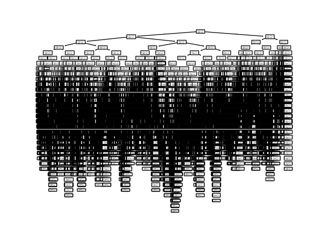
Though we can't read any of the information present, the plot hints at a huge tree. Due to its complexity, the model does not add much value to the understanding of the data (it's simply not interpretable).

Actually visualizing this particular tree takes some time, hence we discouraged you from executing the code.

But why do we get such a huge tree? By default, the CART implementation in scikit-learn grows the tree as large as possible and does not prune it.

... to fix

To prevent the tree from growing too large, we can set two parameters.

from sklearn.tree import DecisionTreeRegressor

# set max_depth and min_samples_leaf
model = DecisionTreeRegressor(
    random_state=784, max_depth=2, min_samples_leaf=15
)

# fit the model again
model.fit(X_train, y_train)

The max_depth parameter limits the depth of the tree, while min_samples_leaf sets the minimum number of samples (observations) required to be in a leaf node. Both prevent the tree from growing too large.

Info

Remember, we want to prevent overfitting. By setting these parameters, we control the complexity of the tree and thus reduce the risk of overfitting. Additionally, it results in a smaller tree which is easier to interpret.

Let's plot the pruned tree.

import matplotlib.pyplot as plt
from sklearn.tree import plot_tree

plot_tree(
    model, 
    filled=True,   # (1)!
    feature_names=X.columns,  # (2)!
    proportion=True  # (3)!
)
plt.show()

1. filled=True colors nodes according to prediction values. A stronger color indicating a higher value.
2. The parameter feature_names is used to label the features in the tree.
3. proportion=True displays the proportion of samples in each node.

Info

Generally, it is always good practice to consult the documentation, if you are unsure about the usage of a function/class.

Regarding plot_tree(), you might find some useful information in the docs that can help you customize the plot to your liking. So don't shy away from reading the documentation!

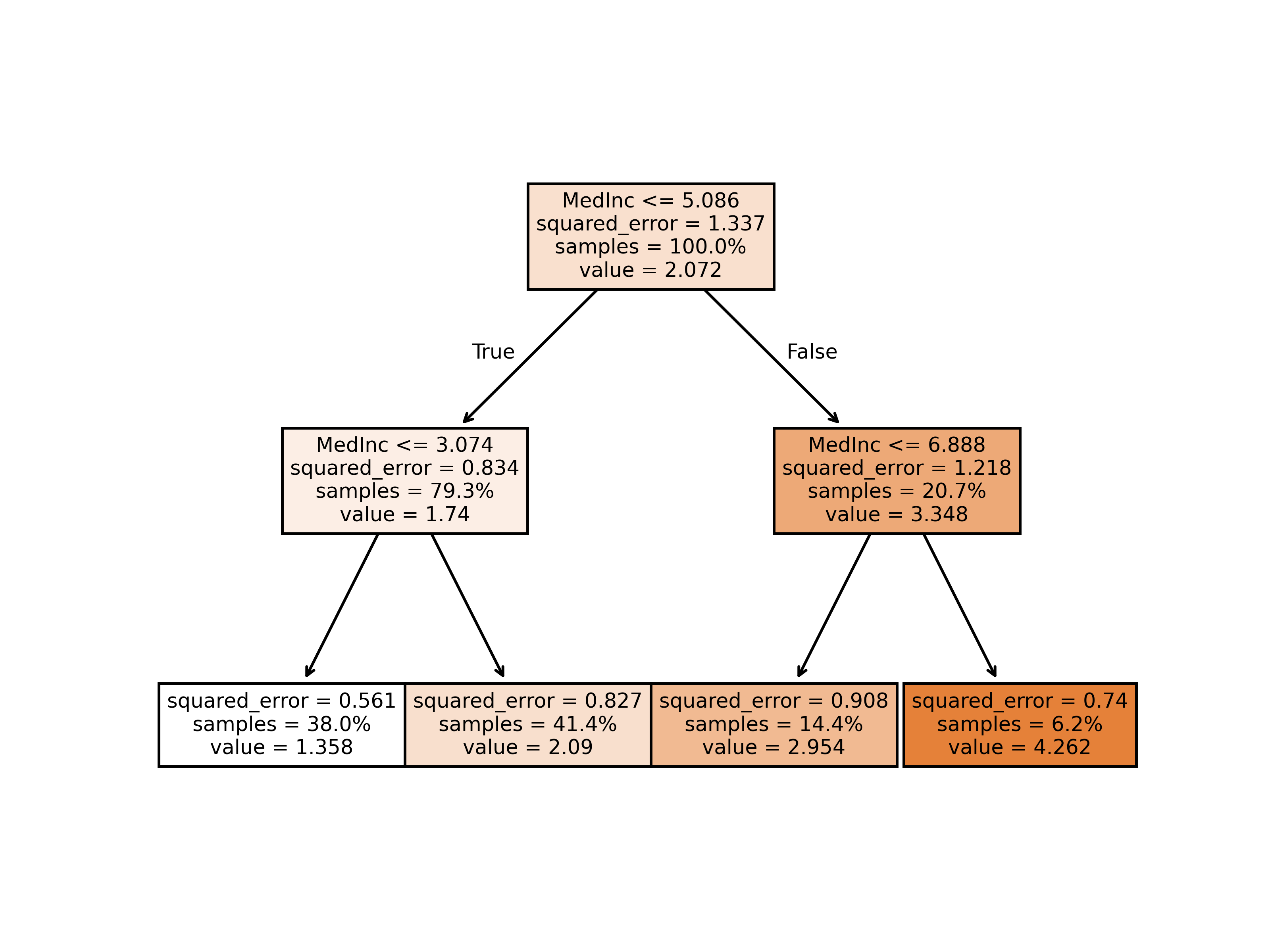The tree is in a stark contrast to the one we had before; it is way smaller.

Tip

The nodes are quite easy to read:

Starting with the root node, the feature MedInc performs the first split. If the median income is less than 5.086, we follow the left branch else the right branch. The resulting squared_error of the split is shown as well. At the root node, the squared_error (sum of the squared differences between the actual values and the predicted value) is 1.337. The lower the squared_error, the better the split. A "perfect split" would result in a squared_error of 0.

The root node splits the data into two subsets, the left branch results in a subest containing 79.3% of the training data and the right branch 20.7%. Compared to the root node, both additional splits lead to a decrease of the squared_error and thus increase the predictive power. After two more splits, we reach the leaf nodes. Each leaf node contains a value, the final prediction.

Now we have a pruned tree, which reduced the risk of overfitting. However, at the cost of model performance. The \(R^2\) decreased from 0.61 to 0.42 which might indicate that such a simple tree might not capture the complexity of the data well.

Now get to the point!

In practice, you have to find the right parameters to balance model complexity and performance. Unfortunately, there is no one-size-fits-all solution. You have to tune the parameters based on the data and the task at hand.

Parameter tuning

Try some different combinations of max_depth and min_samples_leaf. Use the same train test split, we defined earlier.

1. Manually change the values.
2. Fit the model.
3. Evaluate the model.
4. Plot the model.
5. Repeat!

Can you get an \(R^2\) higher than 0.7?

Classification

Next, we switch to a classification task. We will re-use the breast cancer data set introduced in the previous Classification chapter.

Load data

from sklearn.datasets import load_breast_cancer

X, y = load_breast_cancer(return_X_y=True, as_frame=True)
X_train, X_test, y_train, y_test = train_test_split(
    X, y, test_size=0.2, random_state=42, shuffle=True
)

Fit and evaluate the model

For classification trees, scikit-learn provides the class DecisionTreeClassifier.

from sklearn.tree import DecisionTreeClassifier

model = DecisionTreeClassifier(
    # again, set max_depth and min_samples_leaf to prevent growing a huge tree
    random_state=784, max_depth=7, min_samples_leaf=5
)

Fit and evaluate the model

Now it is your time to fit and evaluate the model. Although, you have never used an instance of DecisionClassifier before, you can use the same methods as with other models in scikit-learn. Simply refer to the previous regression example.

1. Fit the model on X_train and y_train.
2. Evaluate the model on X_test and y_test.
3. Print the model's performance.
4. Plot the tree.

Lastly answer following quiz question to evaluate your result.

What is the model's accuracy (rounded to 2 decimal places)?

92.98%

94.74%

90.35%

Submit

Correct! The mean accuracy is 94.74% which is a bit lower than the 95.61% from the logistic regression.

Recap

We comprehensively explored decision trees, focusing on the CART algorithm. The theory section illuminated its core mechanisms, while practical examples demonstrated building and evaluating decision trees for regression and classification tasks. Key takeaways include:

• Algorithm insights into tree construction
• Practical implementation skills
• Understanding of decision trees' interpretability and overfitting risks

Next, we'll extend our knowledge to Random Forests, an ensemble method combining multiple decision trees to enhance predictive performance.

---

1. Christopher M. Bishop. Pattern Recognition and Machine Learning. Springer, 2006. Link ↩↩

2. Leo Breiman, Jerome Friedman, Richard Olshen, and Charles Stone. Classification and Regression Trees. Chapman and Hall/CRC, 1984. https://doi.org/10.1201/9781315139470 ↩

3. scikit-learn documentation: Decision Trees ↩