Clustering
In this section, we will start to explore unsupervised learning, where we work with data that isn't accompanied by labels. One of the primary techniques within this realm is clustering, which aims to uncover patterns or structures in the data by grouping similar data points together. A popular method for achieving this is k-means clustering, which aims to identify clusters of similar observations.
K-means
K-means was briefly introduced in the Introduction to Supervised vs. Unsupervised Learning and used to segment customers based on their annual spending and average basket size.
The algorithm groups similar data points together based on their attributes without being told what these groups should be.
To get a better understanding of k-means, we will explore the theory behind it and employ the algorithm to cluster data from Spotify and a semiconductor manufacturer.
Theory
Info
The theoretical part is adapted from: Christopher M. Bishop. 2006. Pattern Recognition and Machine Learning1
Assume a set of features \(x_1, x_2, ..., x_n\). K-means partitions the data into \(K\) number of clusters. Each cluster is represented by \(\mu_k\), which can be seen as the center of a cluster \(k\).
Intuitively speaking, the goal is to assign each data point \(x_n\) to the cluster with the closest center \(\mu_k\).
The objective
Since, the optimal assignment of data points to specific clusters is not known, the objective is to minimize the sum of squared distances between data points and their assigned cluster centers. This is known as the distortion measure:
Distortion measure
where:
- \(N\) is the number of data points,
- \(K\) being the number of clusters,
- \(r_{nk}\) is a binary indicator of whether data point \(x_n\) is assigned to cluster \(k\),
- \(\mu_k\) representing the cluster center.
In short, we want to find the optimal \(r_{nk}\) and \(\mu_k\) that minimize the distortion measure \(J\).
\(J\) is minimized in an iterative process. First, we initialize \(\mu_k\) with some random values. Then we alternate between two steps:
- Assignment step: Keep \(\mu_k\) fixed. Minimize \(J\) with respect to \(r_{nk}\). This is done by assigning each data point to the closest cluster center.
- Update step: Keep \(r_{nk}\) fixed. Minimize \(J\) with respect to \(\mu_k\). This is done by updating the cluster centers to the mean of the data points assigned to the cluster.
Step 1 can be seen as re-assigning the data points to clusters, while step 2 re-computes the cluster centers.
Info
Since \(\mu_k\) is the mean of the data points assigned to cluster \(k\), we speak of the k-means algorithm.
The optimization of \(J\) is guaranteed to converge, but it might not find the global minimum. The final solution depends on the initial cluster centers.
Get a better understanding
To improve your understanding of the k-means algorithm, either watch the following video or visit the interactive visualization. Both variants illustrate the iterative process of k-means.
Visit the site clustering-visualizer.web.app/kmeans. Use mouse clicks to draw data points. Click on "START".
The web app illustrates the iterative algorithm. You can watch the data points being assigned to clusters and the update of cluster centers which are denoted in the app as \(C_1, C_2, ... , C_N\).
Elbow method 
So far we have not discussed the number of clusters \(K\) in depth. Since the algorithm requires the number of clusters as an input, it is crucial to choose \(K\) wisely.
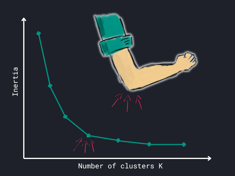
One common approach to determine the optimal number of clusters is the elbow method. The idea is to plot the distortion measure \(J\) (inertia) for different values of \(K\). The plot will show a sharp decrease in \(J\) as \(K\) increases. The optimal number of clusters is the point where the decrease flattens out, resembling an elbow.
We will apply both k-means and the elbow method in the following examples.
Examples
With the theory out of the way, we can now apply k-means to real-world data. First, we build a recommendation system for Spotify tracks and then move on to clustering semiconductor data.
Recommendation system
If you're using a music streaming service, you're familiar with listening to playlist. At the end of a playlist, the service recommends you similar songs based on the previous songs.
We will build such a recommendation system (a rudimentary one) with k-means. The goal is to cluster songs based on their audio features and recommend similar songs to the user.
To build our own recommendation system, we will use a modified Spotify dataset.
Info
The original data can be found on Kaggle.
The modified data we are using, contains songs from 2024 up until now (time of writing: January 31, 2025).
Download and read data
- Download the data set.
- Read it with
pandasand for convenience assign it to a variable calleddata. Then you will be able to use the following code snippets more easily. - Print the first rows of
data.
With the data set loaded, we pick the following audio features for clustering:
features = [
    "danceability",
    "energy",
    "loudness",
    "speechiness",
    "acousticness",
    "instrumentalness",
    "liveness",
    "valence",
    "tempo",
]

# subset data
X = data[features]
Have a look at the data
- Look at the first couple of rows of the
DataFrameX. - Check for potential missing values.
Hint: If you need a refresh on missing values, visit the Data preprocessing chapter.
You might have noticed that all features are numerical. In fact, k-means requires numerical data.
Danger
K-means clustering relies on Euclidean distances, which only make sense for numerical data.
 Never use k-means for categorical data, even if you encode the
categories as numbers or labels. Distances between categorical values
are not meaningful!
Never use k-means for categorical data, even if you encode the
categories as numbers or labels. Distances between categorical values
are not meaningful!
For clustering categorical data, use specialized algorithms like k-modes or other appropriate methods.
Let's have another look at the data:
       danceability        energy  ...       valence         tempo
count  11320.000000  11320.000000  ...  11320.000000  11320.000000
mean       0.683081      0.660006  ...      0.525337    122.571478
std        0.134193      0.162655  ...      0.222797     27.628201
min        0.093900      0.001740  ...      0.000010     46.999000
25%        0.597000      0.560000  ...      0.355000     99.987000
50%        0.701000      0.675000  ...      0.526000    121.974000
75%        0.780000      0.777000  ...      0.696000    140.056000
max        0.988000      0.998000  ...      0.989000    236.089000
These basic statistics reveal that the features have different scales.
For example, compare tempo and danceability. Tempo ranges from
46 to 236, while danceability ranges from
0.0939 to 0.988.
Thus, we apply a Z-Score normalization
to all features (to have a mean of 0 and a standard deviation of 1).
This prevents k-means to disproportionately weigh features like tempo and
ensures each feature contributes equally to the distance calculations.
from sklearn.preprocessing import StandardScaler

scaler = StandardScaler()  # Z-Score normalization
X = scaler.fit_transform(X)
Apply k-means
The application of k-means is straightforward:
from sklearn.cluster import KMeans

kmeans = KMeans(n_clusters=5, random_state=42)
cluster_indices = kmeans.fit_predict(X)
print(cluster_indices)
The n_clusters parameter specifies the number of clusters. We set it to
5 for now. The random_state parameter ensures reproducibility.
Using the fit_predict() method, we obtain the cluster indices for each data
point. In this case, these indices range from 0 to 4.
I.e., the first track belongs to cluster 4, the second to cluster
0, and so on.
... but wait, how do we know if 5 is the right number of clusters?
This is where the elbow method comes into play.
Elbow method
With the attribute inertia_, we can access the distortion measure \(J\).
From the k-means docs:
inertia_:Sum of squared distances of samples to their closest cluster center,...
-- KMeans docs
In a loop we fit the k-means algorithm for different numbers of clusters \(K\)
and store the corresponding distortion measure (inertia_). Then we plot the
results.
We define a function to apply the elbow method:
def elbow_method(X, max_clusters=15):
    inertia = []
    K = range(1, max_clusters + 1)

    for k in K:
        model = KMeans(n_clusters=k, random_state=42)
        model.fit(X)
        inertia.append(model.inertia_)

    # for convenience store in a DataFrame
    distortions = pd.DataFrame(
        {"k (number of cluster)": K, "inertia (J)": inertia}
    )

    return distortions
By default, the function elbow_method() tries values for \(K\) from
1 to 15 and stores the corresponding distortion measure
in a DataFrame.
Apply the elbow method
- Apply the
elbow_method()on our scaled dataX. -
Create a line plot with the number of clusters (K) on the x-axis and the distortion measure on the y-axis.
Hint: Use the
plot()method of the resultingDataFrame.
Expand the below section to see a plot as possible solution.
Expand to see the plot

Choice paralysis
Like in our example, it is not always obvious how many clusters to pick, because the "elbow" can sometimes be subtle or ambiguous. Ideally, you choose the point where the distortion/inertia sharply decreases and then levels off, forming an elbow-like bend in the plot.
In this example, possible candidates for the number of clusters \(K\) are
5, 6 or 7. As we have to make a choice, we
choose 6 clusters.
Now, we have to simply fit the k-means algorithm with n_clusters=6.
 Make recommendations
Now to the fun part!
The goal of this exercise is to recommend a song based on a previous
track. The idea is to pick a song as recommendation that is in the same
cluster as the previous one. To do so, we can use the cluster_indices to
recommend similar songs.
Since the cluster_indices are in the same order as our initial data, we
can simply assign them as a new column.
               spotify_id                name                artists  ... valence    tempo  cluster
0  2plbrEY59IikOBgBGLjaoe    Die With A Smile  Lady Gaga, Bruno Mars  ...   0.535  157.969        4
1  3sK8wGT43QFpWrvNQsrQya                DtMF              Bad Bunny  ...   0.032  136.020        0
2  4wJ5Qq0jBN4ajy7ouZIV1c                APT.       ROSÉ, Bruno Mars  ...   0.939  149.027        2
3  2lTm559tuIvatlT1u0JYG2   BAILE INoLVIDABLE              Bad Bunny  ...   0.219  119.387        0
4  6dOtVTDdiauQNBQEDOtlAB  BIRDS OF A FEATHER          Billie Eilish  ...   0.438  104.978        4
Now, that we assigned a cluster to all 11320 tracks, we can easily
recommend a song based on a given spotify_id (the unique identifier of a
song on the platform).
Use the below functions to see your recommender system in action. Don't worry about the details of these functions.
def print_track_info(track):
    name, artists, cluster = track["name"], track["artists"], track["cluster"]
    print(
        f"Track name: {name}\nArtist: {artists}\nCluster index: {cluster}\n{'-' * 20}"
    )


def recommend_track(spotify_id, data):
    """Get a recommendation for a given spotify_id."""

    # info about previous track
    previous_track = data[data["spotify_id"] == spotify_id].squeeze()
    # get the cluster index of the previous track
    cluster_index = previous_track["cluster"]

    print("Your previous track:\n")
    print_track_info(previous_track)

    # pull all tracks from the cluster
    recommendation = data[data["cluster"] == cluster_index]
    # exclude the previous track
    # (we do not want to recommend the same track again)
    recommendation = recommendation[recommendation["spotify_id"] != spotify_id]

    # pull a random sample from the cluster
    recommendation = recommendation.sample(1).squeeze()

    print("Your recommendation:\n")
    print_track_info(recommendation)
Pick any spotify_id from the data set (data) to start recommending songs.
recommend_track() will pick a song that is in the same cluster.
Your previous track:

Track name: Wake Me Up (feat. Justice)
Artist: The Weeknd, Justice
Cluster index: 4
--------------------
Your recommendation:

Track name: Aarre
Artist: Ultra Bra
Cluster index: 4
--------------------
Recommend more songs
Every time you run the recommend_track() function, you will get a new
recommendation. Try it out!
- Pick another
spotify_idand recommend a song. - Repeat the process a couple of times.
Are the recommendations good?
As you've tried the recommender system a couple of times, you might have
wondered if the recommendations are actually good?!

Simply put, you have to be the judge if we were actually able to cluster similar songs together and build a good recommendation system.
In this application, it's quite intuitive: If you as a user like the recommendations and keep listening to the recommended songs, the system is successful.
Info
When talking about supervised tasks, we were able to measure the performance of our models. However, in unsupervised learning, like clustering, we do not have labels to compare our results to. Thus, evaluating the performance of unsupervised learning methods is challenging.
In practice, you have to rely on domain knowledge to interpret the results and assess the quality of the model.
Semiconductor data
K-means is not only useful for recommendation systems, but also for anomaly detection. The idea is to form clusters which in turn can be used to detect the outliers/anomalies.
Info
The data is adapted from the UCI Machine Learning Repository.2
In this example, you will apply k-means to semiconductor data.
Download and read data
- Download the below data set.
- Read it with
pandas. - Have a look at the data.
Each row in the data set
represents a single production entity with associated measured features [...]
-- UCI Machine Learning Repository
Apply k-means
Solve the following tasks to apply k-means to the semiconductor data:
- Are there any missing values in the data?
- Deal with potential missing values; choose any suitable strategy. We
recommend to utilize the
SimpleImputerwith your chosen strategy. The application of theSimpleImputershould be straightforward as it implements the methods you already know, e.g.,fit_transform(). - Do you need to scale the features? If so, apply a
StandardScaler. - Use the elbow method to determine the number of clusters.
- Fit the k-means algorithm with the optimal number of clusters.
Hint: You can reuse the functions and code snippets from the Spotify example.
Info
If you have solved the above tasks, you might wonder how to interpret your clustering results. Moreover, how can you detect potential anomalies?
Again, it all depends on domain knowledge. If you're a expert in the semiconductor industry you might be able to tell if the clusters make sense and if there are any anomalies in the data. Otherwise, interpretation can be quite challenging.
Recap
In this chapter, we introduced k-means clustering. We covered the theory followed by two practical examples: building a recommendation system for Spotify tracks and clustering semiconductor data.
We employed the elbow method to determine the optimal number of clusters and discussed the challenges of evaluating clustering results.
In the upcoming chapter, we introduce another unsupervised method, namely Principal Component Analysis (PCA) to reduce the dimensionality of data. PCA can be useful in various ways:
- reducing the computational complexity of algorithms
- visualizing high-dimensional data in a 2D or 3D space
Especially the latter can aid in interpreting the results of clustering algorithms.
-
Christopher M. Bishop. Pattern Recognition and Machine Learning. Springer, 2006. Link ↩
-
McCann, M. & Johnston, A. (2008). SECOM [Dataset]. UCI Machine Learning Repository. https://doi.org/10.24432/C54305 ↩