Dimensionality Reduction
Principal Component Analysis (PCA)
In data science and machine learning, we often encounter data sets with hundreds or even thousands of features. We speak of high-dimensional data sets. While these features may contain valuable information, working with such high-dimensional data can be computationally expensive, prone to overfitting, and difficult to visualize. This is where another unsupervised method, dimensionality reduction comes in — a technique used to simplify data sets, while retaining much of the critical information.
One of the most widely used methods for dimensionality reduction is Principal Component Analysis (PCA). PCA transforms a high-dimensional (= lots of features) data set into a smaller set of features (components). In practice, PCA can reduce hundreds of features down to just 2 or 3 features, making PCA an ideal tool for visualization, preprocessing, and feature extraction.
In this section, we will explain the inner workings of PCA and apply it to the semiconductor data set.
What is PCA?
PCA is a linear transformation technique that identifies the directions (also called principal components) in which the data varies the most. These principal components capture as much variance as possible. PCA has a variety of applications, such as:
- Data visualization: Plot a dimensionality reduced data set in 2D.
- Preprocessing: Removing noise or redundant features while retaining the essential patterns in data.
- Feature engineering: Summarizing high-dimensional data into a smaller set of meaningful features.
How does it work?
PCA follows these essential steps:
-
Compute the covariance matrix: PCA captures relationships between features by calculating the covariance between them.
Info
Think of the covariance matrix as the "spread" of the data. PCA looks at the interaction the correlation of features with each other. Visit the correlation chapter in the statistics course to learn more about covariance.
-
Eigen decomposition: Identify the eigenvalues and eigenvectors of the covariance matrix. The eigenvectors represent the directions of the principal components, while the eigenvalues represent the amount of variance captured by each component.
Info
If you want to know more about eigenvalues and eigenvectors, check out this site.
-
Rank components: Components are ranked by their eigenvalues. The first principal component captures the most variance, the second captures the next-most, and so on.
- Transform the data: Project the original data onto the top principal components to reduce its dimensionality.
The mathematical objective
Let’s assume we have a data set \(X\) with \(p\) features (dimensions). We aim to transform \(X\) into a new matrix \(Z\) with \(k\) features such that \(k < p\), while retaining as much variance as possible.
The transformation (described previously under point 4) is defined as:
PCA transformation
Where:
- \(Z\) is the transformed data set in the lower-dimensional space,
- \(W\) is a matrix whose columns are the top \(k\) eigenvectors of the covariance matrix of \(X\).
Tip
Dimensionality reduction helps in combating the curse of dimensionality, a phenomenon where the performance of algorithms deteriorates with an increase in the number of features. Algorithms like clustering often struggle to find meaningful patterns when working with a high-dimensional data set.
Example
It’s time to apply PCA to real-world data. We'll revisit the semiconductor data set that we used in the previous clustering chapter. The first goal is to use PCA to reduce the data set's dimensions and visualize them.
Prepare the data
First, we load the data set. If you haven’t already downloaded it, you can grab it below:
Load the data
- Load the
csvfile and assign it to a variable calleddata.
Before applying PCA, let’s make sure we deal with potential problems such as missing values.
Next, scale the features to standardize the data set to ensure that all features contribute equally to the analysis, preventing features with larger numerical ranges from dominating the principal components.
from sklearn.preprocessing import StandardScaler

scaler = StandardScaler()  # Z-Score
scaled_data = scaler.fit_transform(data)
Apply PCA
We now apply PCA to reduce the dimensions. First, we fit the PCA model on
the scaled_data:
from sklearn.decomposition import PCA

pca = PCA(n_components=2, random_state=42)  # (1)!
components = pca.fit_transform(scaled_data)
- Although the above definition of PCA is deterministic, the actual
implementation can be stochastic (depending on the solver used). Since
svd_solveris set to"auto"by default, the results can vary slightly. Long story short, settingrandom_stateensures reproducibility in all cases.
n_components=2 specifies that we want to reduce the data set to 2 dimensions.
Check the shape
- What is the shape of the
componentsarray?
Visualize
We can easily visualize the low-dimensional data set using a scatter plot:
import matplotlib.pyplot as plt

components = pd.DataFrame(components, columns=["PC1", "PC2"])
components.plot(kind="scatter", x="PC1", y="PC2", alpha=0.5)  # (1)!
plt.show()
- The
alphaparameter controls the transparency of the points. A value of0.5makes the points semi-transparent.

To quickly recap so far:
We were able to reduce the semiconductor data set from 590
features to just 2.
Plot interpretation
The scatter plot shows the data set in a 2D space with each observation as a point. Additionally, we can observe clusters. Since, principal components are ranked by the amount of variance they capture, the first component (PC1) is "more important" than the second component (PC2).
Therefore, differences along the x-axis (PC1) are more significant than differences along the y-axis (PC2). As we are interested in potential anomalies in semiconductor products, we can detect some observations that might be well worth some further investigation:
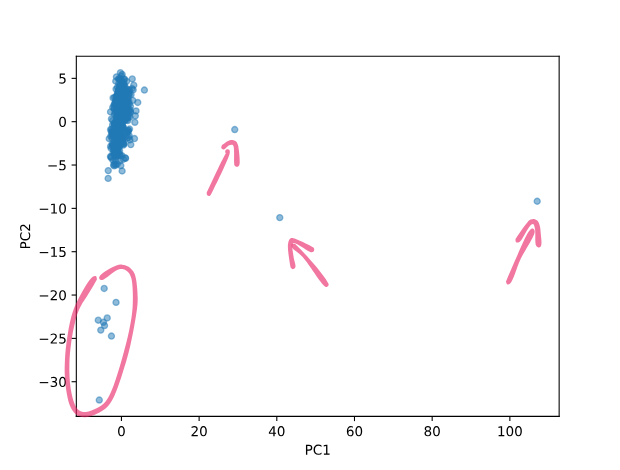
A majority of the data points are clustered in the upper left corner. Contrary, these single observations with a high difference on the x-axis (PC1) might be anomalies (annotated by these arrows). Although, samples within the encircled area have their differences on the y-axis (PC2), they are still worth investigating.
Re-apply PCA on unscaled data
What would happen if you apply PCA to the unscaled data?
- Create a new PCA instance with
n_components=2. - Fit the PCA model on the
data(unscaled) and transform it. - Visualize the new components in a 2D scatter plot.
- Compare the results with the previous PCA visualization.
Tip
PCA is sensitive to the scale of the data. Thus, the scaled data nicely separates the clusters, while the unscaled data does not. So be sure to pick the right preprocessing steps for your data.
Explained variance
When evaluating a PCA model, it is crucial to understand how much variance is
captured by each principal component. Simply access the
explained_variance_ratio_ attribute:
Regarding, the pca fitted on the scaled data, the output is:
The first principal component captures approximately 6.32% of the variance,
while the second component captures 3.67%. Together, the two components
capture roughly 10% of the variance.
Tip
Put simply, our two principal components capture 10% of the variance
of the original 590 features which is not that great.

Unfortunately, when dealing with real world data, results may not be as promising as expected. In this case, we might need to consider more components to capture a higher percentage of the variance.
Choosing the number of components
It is essential to choose the right number of components. For example, you could use the components as features for another machine learning model, hence you want to retain as much information as possible.
However, the choice of how many components to keep is subjective. A common approach is to retain enough components to explain 90-95% of the variance.
Number of components to exceed 95% variance
Using the scaled semiconductor dataset:
- Create a PCA model to analyze the variance in the data
- Determine the minimum number of principal components needed to explain at least 95% of the total variance
Solution approaches:
- You can use the
explained_variance_ratio_attribute, OR - There is an alternative approach that requires only 3 lines of code maximum (hint: google and check the PCA documentation)
Use the following quiz question to evaluate your answer.
How many components are necessary to explain at least 95% of the variance?
Bonus: PCA & k-means combined
In the previous chapter, we applied k-means clustering to the semiconductor data set. Now, we can combine PCA and k-means to cluster the data set in a lower-dimensional space. This approach can help us plot the clusters in a 2D space.
With the elbow_method() from the previous chapter we provide an end-to-end
solution.
elbow_method()
def elbow_method(X, max_clusters=15):
    inertia = []
    K = range(1, max_clusters + 1)

    for k in K:
        model = KMeans(n_clusters=k, random_state=42)
        model.fit(X)
        inertia.append(model.inertia_)

    # for convenience store in a DataFrame
    distortions = pd.DataFrame(
        {"k (number of cluster)": K, "inertia (J)": inertia}
    )

    return distortions
Read and run the code
Be sure to read, run and comprehend the code below.
To summarize, we applied the same preprocessing steps, reduced the data to
2 dimensions using PCA. Afterward, we called the elbow method on the 2
components to determine the optimal number of clusters. Then we applied
k-means with n_clusters=5. Finally, we plot the 2 components and
color the observations according to their corresponding clusters. Have a look
at the resulting plots.

The plot shows the semiconductor data set clustered into 5 groups. Each color represents a different cluster. The clusters are well separated in the 2D space.

The plot shows the distortion (inertia) for different numbers of
clusters. This time around, we can distinctly see an elbow at k=5
clusters. 
Recap
In this chapter, we concluded the Supervised vs. Unsupervised Learning portion of this course and introduced Principal Component Analysis (PCA), a linear technique for dimensionality reduction.
We discussed the inner workings of PCA and applied it to the semiconductor data set, where we could identify potential anomalies in the data. We also visualized the data set in a 2D space, making it easier to interpret and analyze. Lastly, a combination of PCA and k-means revealed distinct clusters in the semiconductor data set.