Detection
After learning about computer vision in general and how YOLO works, we can start using YOLO for our purposes. We will see, how much we can do with little code.
Project Setup
We start with the project structure from before and create a new jupyter notebook yolo_detect.ipynb
.venv) is selected and all needed packages (ultralytics) are installed.
Now we can download our test pictures, extract the ZIP file and save it in the 📁 pics/ folder.
Now we are all set for our first detection 🎉
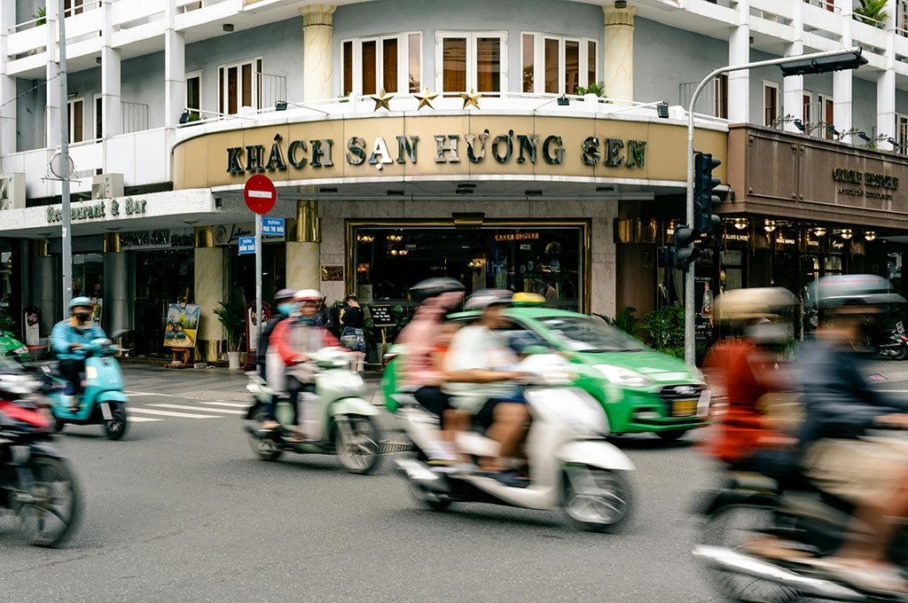
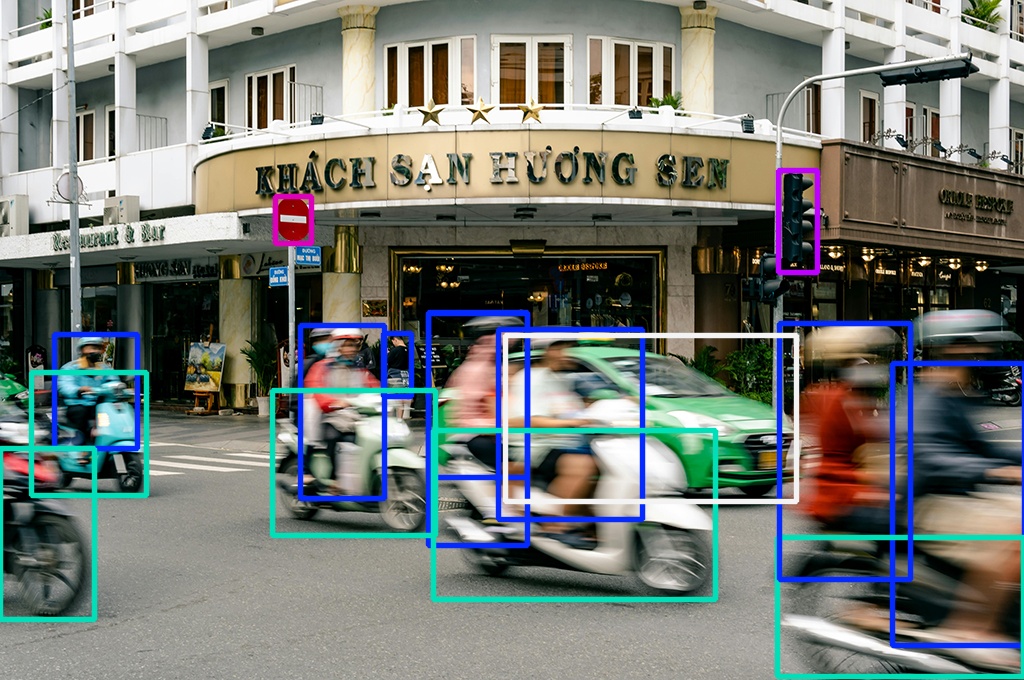
We will start with the picture pic2.jpg which is quite challenging due to motion blur.
Inference
Inference
In machine learning, inference refers to the process of using a trained model to make predictions or decisions on new, unseen data. It's the production phase where the model applies what it learned during training to analyze new inputs and generate outputs, like when a trained image recognition model identifies objects in a new photo.
Pretrained Models
Fortunately, so that we don't have to start from scratch, there are already pre-trained models from YOLO that we can use. These pre-trained models have been trained with the help of a lot of data (for detection e.g. on the COCO dataset) and are now available to us without any further effort. For example for detection:
| Model | size (pixels) |
mAPval 50-95 |
Speed CPU ONNX (ms) |
Speed T4 TensorRT10 (ms) |
params (M) |
FLOPs (B) |
|---|---|---|---|---|---|---|
| YOLO11n | 640 | 39.5 | 56.1 ± 0.8 | 1.5 ± 0.0 | 2.6 | 6.5 |
| YOLO11s | 640 | 47.0 | 90.0 ± 1.2 | 2.5 ± 0.0 | 9.4 | 21.5 |
| YOLO11m | 640 | 51.5 | 183.2 ± 2.0 | 4.7 ± 0.1 | 20.1 | 68.0 |
| YOLO11l | 640 | 53.4 | 238.6 ± 1.4 | 6.2 ± 0.1 | 25.3 | 86.9 |
| YOLO11x | 640 | 54.7 | 462.8 ± 6.7 | 11.3 ± 0.2 | 56.9 | 194.9 |
Running the Detection
Based on these pretrained models, to detect objects in an image with YOLO, only a few lines of code are required:
# Import required librarys
from ultralytics import YOLO

# Define the path to the source picture
picpath = "pics/pic2.jpg"

# Load a pretrained YOLO11 Model (Size: Nano)
model_det = YOLO("yolo11n.pt")

# Apply the model to our source picture
results = model_det(picpath)
image 1/1 c:\path\to\pics\pic2.jpg: 448x640 6 persons, 1 car, 5 motorcycles, 1 traffic light, 1 stop sign, 40.3ms
Speed: 2.0ms preprocess, 40.3ms inference, 0.0ms postprocess per image at shape (1, 3, 448, 640)
And that's it! Your performed your first detection.
Analyzing the Output
Now we can take a closer look at the different parts of the output:
-
Information about the image:
-
image 1/1 c:\path\to\pics\pic2.jpg: 448x640This includes the path to the image and the image size YOLO uses for the detection (this is not the original image size)
-
shape (1, 3, 448, 640)batch size (number of pictures):
1picture channels:
3(RGB)picture hight:
448picture width:
640
-
-
Detected objects:
6 persons, 1 car, 5 motorcycles, 1 traffic light, 1 stop sign
-
Speed Metrics:
Speed: 2.0ms preprocess, 40.3ms inference, 0.0ms postprocess per image
But are those all of the results? Where are those objects in the image? How sure are we, that there are six persons? We need to go deeper into the results.
Understanding the results
The before seen output of the detection is just a brief overview. All the information is stored in results
Task: Analyze the Results
Take a look at the result and answer the following questions (don't forget to use google and the docs)
- What is the original shape of the image?
- How many different classes are available and what are they?
- Why is
keypoints,masksandobbNone? What do you think?
Now go deeper and analyze result.boxes
- What are the detected classes? How do they respond to the labels (person, car,...)
- How sure is YOLO about the detected objects? (hint: the right wording is confidence)
- What are the differences between
xywh,xywhn,xyxyandxyxyn datais the collection of what?- How are
dataandshapeare connected?
Multiple Images
You can also pass multiple images at once. To access the results for a specific image, you need to choose one from the results list.
Now, that we are familiar with the results, we can write a little function to print a more detailed overview:
def print_overview(result):
    # Print object count
    print(f"Detected {len(result.boxes)} objects")

    # Examine each detection
    for box in result.boxes:
        # Get class name
        class_id = int(box.cls)
        class_name = model_det.names[class_id]

        # Get confidence
        confidence = float(box.conf)

        # Get coordinates (x1, y1, x2, y2 format)
        x1, y1, x2, y2 = box.xyxy[0].tolist()

        print(f"\nDetection:")
        print(f"- Class: {class_name}")
        print(f"- Confidence: {confidence:.2f}")
        print(f"- Coordinates: ({x1:.1f}, {y1:.1f}) to ({x2:.1f}, {y2:.1f})")

print_overview(result)
Detected 14 objects

Detection:
- Class: motorcycle
- Confidence: 0.81
- Coordinates: (2177.1, 3142.4) to (3490.8, 4281.8)

Detection:
- Class: motorcycle
- Confidence: 0.75
- Coordinates: (0.0, 3574.5) to (755.0, 4952.4)

...
So far we have everything we need to detect objects in images and work with the results.
But sometimes a picture is worth a thousand words!
Visualize the Results
In some cases, the 'simple' extraction of the results is not sufficient and a visualization is needed.
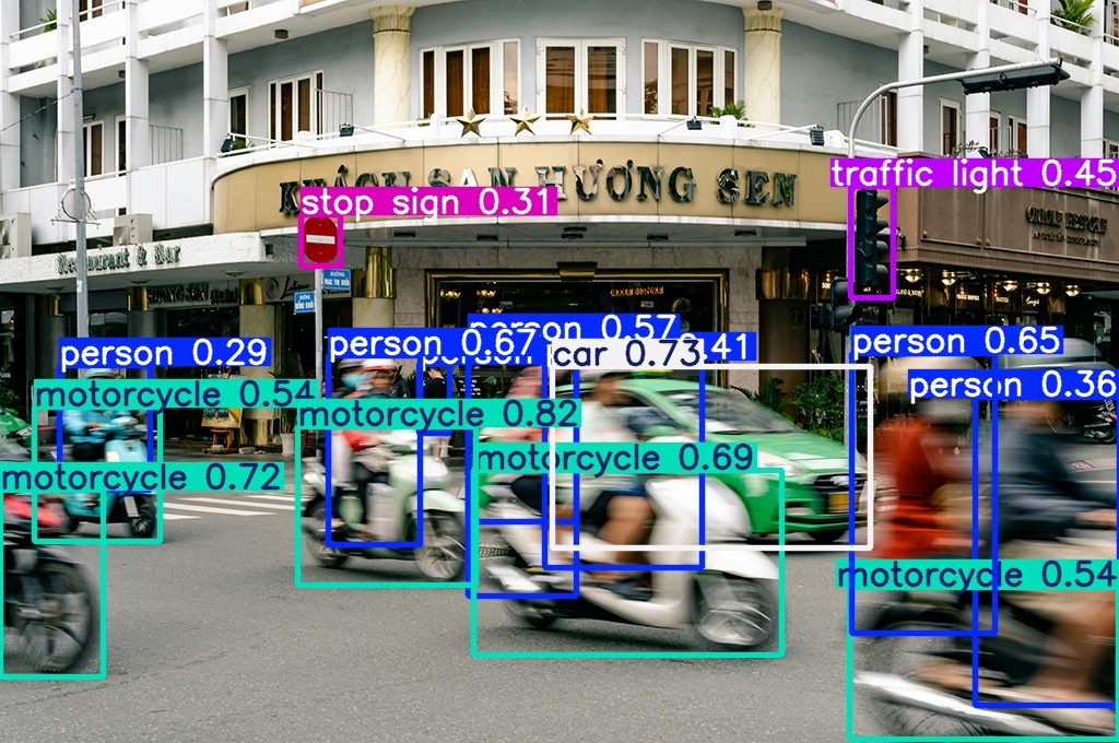
For visualizing the results there are two options available: showing and saving the picture.
Showing the Resulting Image
YOLO makes it really easy to show the resulting image. With the method .show() the result can be visualized:
This should result in the above shown image.
Saving the Resulting Image
There are multiple ways to save the resulting image.
Saving Images
YOLO offers various visualization arguments, which can be used directly in the inference command. One of them is save=True
Unless other specified, the file will be saved in a new folder 📁 runs/detect/predict/. Use the argument save_dir='your/custom/path' to specify a different folder.
When you install ultralytics the package opencv-python will be installed automatically as dependency. openCV is a powerful tool for image and video processing and can also be used for saving the image
annotated_image = result.plot()

# Display using OpenCV
import cv2

# Save the image
cv2.imwrite("output_detection.jpg", annotated_image)
📁 computer_vision.
See the Magic Happen
If you are interessted in seeing, what the model is seeing and doing, you can use another visualization argument
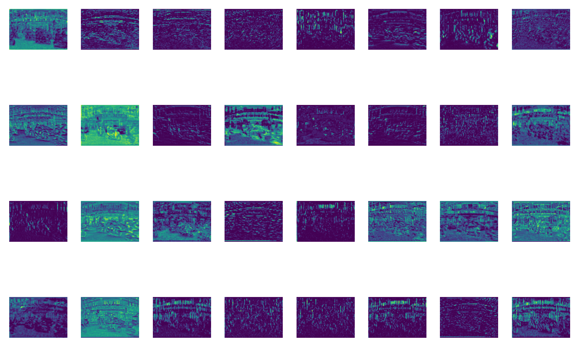
The resulting pictures in the folder 📁 runs/detect/predict/pic2 are a 'Intermediate Features Visualization'
- This parameter saves visualizations of the intermediate feature maps or activations from the YOLO model.
- These feature maps show what parts of the image the model focuses on during different stages of the neural network.
- These outputs help in debugging and understanding the model's inner workings.
Inference Arguments
After we worked on the output side of the Yolo, it's now time to focus more on the input side. Besides those visualization arguments we have used before, there are numerous inference arguments, which can be handed over to the model. An overview can be found in the documentation
Task: Inference Arguments
- Confidence
- Run a detection with confidence threshold 0.5.
- Save this image as
high_conf.jpg - Now try confidence 0.25, save as
low_conf.jpg - Compare both images - what differences do you notice?
- What is the default value?
- Classes
- Limit your detection to just detect
motorcycleandcar - Save the results as
class_limit.jpg
- Limit your detection to just detect
- Adjusting the output path
- Use the two inference arguments
projectandnameto adjust the output folder to📁 output_pics/detection_pics/.
- Use the two inference arguments
- Adjust the visual outcome
- Run a detection for our
pic2.jpgimage and adjust:- no label should be shown
- no confidence should be shown
- line width of the boxes should be 3
- Run a detection for our
Further Adjustments
As we have discussed before, YOLO comes in different model sizes, trading speed for accuracy.
Task: Model Comparison
For each model size determine the following characteristics by running a detection on the pic2.jpg:
- Time the detection speed
- Count detected objects
- Compare confidence scores
- Create a table with your findings:
| Model | Detection Time | Objects Found | Avg Confidence |
|---|---|---|---|
| nano | |||
| small | |||
| medium | |||
| large | |||
| extra large |
🎉 Congratulations
You are now able to perform object detection on images and work with the results!
